The elementary kriging approximation is that the global temperature anomaly (TG) is a proportional mix of the ocean temperature (To) with the land temperature (Tl ):
$$ T_G = p_o T_o + p_l T_l $$
where
$$ 1 = p_o + p_l $$
with the approximate fraction of earth's coverage by the ocean equal to 0.7 (and the land therefore 0.3).
We use that Hadley center data sets
| global | land | ocean |
|---|---|---|
| hadcrut4 | crutem4vgl | hadsst2gl |
Shifting the baseline anomaly by at most 0.1C, we come up with the following fit, shown in Figure 1. The composed temperature lines up very closely to the reported global temperature, with the red areas peeking out where the agreement is not perfect.
 |
| Figure 1 : Global temperature anomaly is straightforwardly recreated by assuming that the global temperature is composed by a proportion of ocean and land area. The fit works very well apart from a few points (years centered around 1948) that may be traced to systemic errors or discrepancies the database versions. |
That by itself is only somewhat interesting, as it merely confirms that the Hadley center researchers know how to do first order proportional mapping (aka kriging). The regression agreement is shown in Figure 2.
 |
| Figure 2 : The composed temperature maps nearly one-to-one to the actual global temperature. |
The other identity we need to consider involves a fraction of the heat sunk by the ocean. Since the land has essentially no heat sink, but that the ocean has a fraction f that acts as a heat sink, we can assert:
$$ T_o = f T_g $$
where we determined previously that f is about 0.5.
We can plot the linear regression between the two below.
 |
| Figure 3 : Linear regression between Land and SST temperature is more noisy. |
As this is fit is fairly noisy, we can try to reduce the variance by plotting against the global mean temperature as a multiple regression fit. We take the first equation and replace each of the component temperatures with their fractional equivalents.
$$ T_G = p_o f T_l + p_l T_l $$
$$ T_G = p_o T_o + p_l \frac{T_o}{f} $$
and then apply these as equal weightings
$$ T_G = 1/2 ( p_o f T_l + p_l T_l ) + 1/2 ( p_o T_o + p_l \frac{T_o}{f} )$$
$$ T_G = 1/2 ( f p_o + p_l ) T_l + 1/2 ( p_o + \frac{p_l}{f} ) T_o $$
If we apply a multiple regression of the global temperature data against a linear combination of the ocean and temperature data we get the following tabulated results:
| Coefficients | Standard Error | t Stat | P-value | Lower 95% | Upper 95% | |
| Intercept | 0.02225179 | 0.003884172 | 5.728838 | 4.97E-08 | 0.0145802 | 0.02992339 |
| Land | 0.29922517 | 0.015995888 | 18.70638 | 6.56E-42 | 0.26763182 | 0.33081852 |
| Ocean | 0.65796939 | 0.024637656 | 26.70584 | 1.86E-60 | 0.60930775 | 0.70663103 |
With this information, we can solve for f and the land ocean split.
$$ 1/2 ( f p_o + p_l ) = 0.299 $$
$$ 1/2 ( p_o + \frac{p_l}{f} ) = 0.658 $$
Given two linear equations and two unknowns, we get f = 0.46 and ocean fraction of 73.5%.
The solution is also shown as the open circles in Figure 1.
We originally asserted that 1/2 the heat is entering the ocean, and substantiated this with a value of 0.46. We can also compare the generally agreed upon value of 71% of the surface water coverage with the value of 73.5% determined here. Given the confidence interval uncertainty in the coefficients as shown in the table above, we see that this simple analysis substantiates our original premise.
This is also a subtle effect and can easily be misinterpreted as arising from just the proportional warming of ocean and land. However something has to create the temperature imbalance between the ocean and land, and the fact that the coefficients of proportionality shown in the table come out fairly close to 0.3 and 0.7 (those of land and ocean) is just a coincidence in the math. If some value markedly different from 0.5 for heat sinking was involved, then the ratios would differ more obviously.
Climate science, like other science disciplines, consists of an array of interlocking parts that need to fit together. If these don't fit, our model will lose its predictive power. In the case of this model, we can help verify that the excess heat is entering the ocean, suppressing the global temperature by about 2/3 from the land temperature. This will continue as long as the ocean acts as a heat sink, a point still some distance in the future. All we can really say is that global temperature anomalies have the potential for increasing by 3/2 or by 50% from the current readings when they eventually and asymptotically reach a near-equilibrium steady-state.
UPDATE
Using the Eureqa curve fitting software, a linear combination of data sets provides the low complexity fit.
 |
| Figure 4: The linear combination of SST and Land with an offset gives a Pareto frontier optimum |
It's the ocean heat content, stupid
June 22, 2013. This paper has applicability to the proportional land/sea warming model
The research results claim that the ocean has been adjusting its heat uptake in the last few years as a result of transient changes in the large-scale hydrodynamics. This has the effect of suppressing the warming in terms of temperature, although the heat uptake from the AGW forcing still exists. So the implication is that what is lacking in a temperature rise is made up for by the heat sinking of the ocean (also see the "missing heat" issue studied by Trenberth).M. Watanabe, Y. Kamae, M. Yoshimori, A. Oka, M. Sato, M. Ishii, T. Mochizuki, and M. Kimoto, “Strengthening of ocean heat uptake efficiency associated with the recent climate hiatus,” Geophysical Research Letters, 2013.
The ocean heat uptake efficiency measure of Watanabe is related to the ratio f between ocean and land temperature defined at the top of this post. The idea is that -- similar to the aim of the Japanese research study -- to see if we can detect changes in f over the last few years.
To do this we need to take great care with the numbers. Instead of using the WoofForTrees data, I used the CRU data directly. The sets were CRUTEM4 (land), HadCRUT4 (global), and HadSST3 (sea). The composed set looks like the following chart for a value of f = 0.5, which is the nominal fraction assumed for the original proportional land/sea analysis.
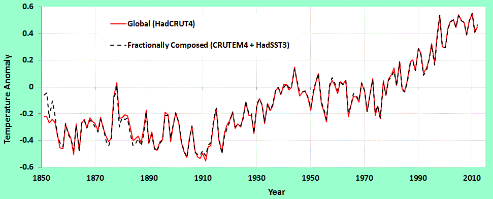 |
| The composed temperature lies on top of the HadCRUT4 global temperature |
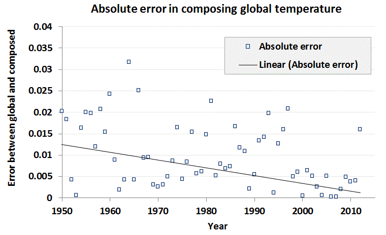 |
| The absolute error decreases with more recent records. (The last data point is 2012, which often undergoes corrections for the next update.) |
The high resolution and low error in recent years indicates that perhaps we can try to more accurately fit the fraction f. So essentially, we want to zero out the error by solving the proportional land/sea warming model for a continuously varying value of f.
$$ 0 = T_G - 1/2 ( f p_o + p_l ) T_l + 1/2 ( p_o + \frac{p_l}{f} ) T_o $$
This turns into a quadratic equation for f, which we can solve by the quadratic formula. The set of value calculated by minimizing the error is shown below. Note that the average remains around f = 0.5, but it shows a distinct decreasing trend in recent years.
 |
| The fraction ratio of ocean to land temperature appears to be decreasing in recent years, leading to an apparent flattening in global temperature rise. Lower values of f cause the global temperature signal to appear cooler for a given AGW forcing. |
If this is a real trend (as opposed to some type of accumulating systemic error or noise) it is telling us that more of the heat is accumulating in the ocean, consistent with the claims of Watanabe et al. It is possible that the fraction is actually decreasing from a past value of around 0.6 to a current value of 0.4. Although this is a subtle effect in terms of the fit (probably the not most robust metric one can imagine), it has significant effect in terms of the global surface temperature signal.
This is seen if we deconstruct the proportional model in terms of the land temperature alone, assuming the area land/ocean split as 0.71/0.29 :
$$ T_G = (0.71 \cdot f + 0.29 ) T_l $$
Note that with a slowly increasing land temperature signal Tl , the declining f can compensate for this value and actually cause the global temperature value TG to flatten.
To take an example, reducing the value of f from 0.6 to 0.4 causes the global temperature to decline from 0.716*Tl to 0.574*Tl. If the land temperature is held constant, the global temperature will decline, while if the land temperature rises by 25%, the global temperature rise will look flat.
 |
| Contour plot showing optimal values of f. This is a log plot and higher negative values indicate low error |
That is exactly what Watanabe et al are claiming. Moreover, they assert that this decline can't remain in place for the long term, and eventually the ocean hydrodynamics will stabilize or even reverse, with a concomitant rebound in global temperature.
To review, the essential premise of the proportional land/ocean model is:
- The land surface reaches the steady-state temperature quickly
- The ocean sinks excess heat, thus moderating the sea surface temperature rise.
- The fractional ratio of ocean temperature to land temperature is given by f.
- The global surface temperature is determined as combination of land and sea surface temperatures prorated according to the land/sea areal split.
(also see I. Held's blog post on this topic [2])
References
[1]
D. Dommenget, “The ocean’s role in continental climate variability and change,” Journal of Climate, vol. 22, no. 18, pp. 4939–4952, 2009.
“The land–sea warming ratio in the ECHAM–HadISST holds also for the warming trend over the most recent decades, despite the fact that no anthropogenic radiative forcings are included in the simulations. The temperature trends during the past decades as observed and in the (ensemble mean) model response (Fig. 4) are roughly consistent with each other, which indicates that much of the land warming is a response to the warming of the oceans. The simulated land warming, however, is weaker than that observed in many regions, with an average land–sea warming ratio of 1.6, amounting to about 75% of the observed ratio of 2.1 .”
[2]
I. Held, “38. NH-SH differential warming and TCR « Isaac Held’s Blog.” [Online]. Available: http://www.gfdl.noaa.gov/blog/isaac-held/2013/06/14/38-nh-sh-differential-warming-and-tcr/#more-5774. [Accessed: 25-Jun-2013].
No comments:
Post a Comment