I am always motivated to find simple relationships that expose the seeming complexity of the climate system. In this case it involves the subtly erratic behavior observed in paleoclimate temperature versus CO2 data. The salient trends are there, in that CO2 and Temperature track each other, but the uncertainties cause climate watchers some puzzlement. The following tries to put a model-based understanding to what I think is happening. As usual, this does not rely on detailed climate models but simply pragmatic physical considerations placed in a mathematical context.
Premise. A model of long-term global temperature and CO2 interactions would assume two primary contributions.
First, we have the forcing function due to the greenhouse gas properties of atmospheric CO2 concentrations, where c = [CO2] is in parts per million (PPM). The first-order paramater alpha, α, is known as the climate sensitivity and is logarithmic with increasing concentrations (log=natural log): $$ \Delta T = \alpha \log {\frac{[CO_2]}{C_0}} $$ The second contributing factor is due to steady-state outgassing of CO2 from the ocean's waters with temperature. A first-order approximation is given by the Arrhenius rate law to estimate gaseous partial pressure. The standard statistical mechanical interpretation is the invocation of a Boltzmann activation energy to model the increase of steady-state pressure with an increasing temperature bath. $$ p = p_0 e^{\frac{-E_a}{kT}} $$ To keep things simple we use the parameter beta, β, to represent the activation energy in Kelvins, where k is Boltzmann's constant. The relation between Kelvins and electron volts is 11600 Kelvins/eV. $$ \beta = \frac{E_a}{k} $$ $$ p = p_0 e^{\frac{-\beta}{T}} $$ This works very well over a reasonable temperature range, and the activation energy Ea is anywhere between 0.2 eV to 0.35 eV. The uncertainty is mainly over the applicability of Henry's law, which relates the partial pressure to the solubility of the gas. According to a Henry's law table for common gases, the CO2 solubility activation energy is β = 2400 Kelvins. However, Takahashi et al (see reference at end) state that the steady state partial pressure of CO2 above seawater doubles with every 16 celsius degree increase in temperature. That places the activation energy around 0.3 eV or a β of 3500 Kelvins. This uncertainty is not important for the moment and it may be cleared up if I run across a definitive number.
Next, we want to find the differential change of pressure to temperature changes. This will create a limited positive feedback to the atmospheric concentration and we can try to solve for the steady-state asymptotic relationship. The differential is: $$ d[CO_2] \sim dp = \frac{\beta}{T^2} p dT \sim \frac{\beta}{T^2} [CO_2] d\Delta T $$ In terms of a temperature differential, we invert this to get $$ d\Delta T = \frac{T^2}{\beta [CO_2]} \Delta [CO_2] $$ Now we make the simple assertion that the differential changes in temperature will consist of one part of the delta change due to a GHG factor and another part due to the steady-state partial pressure. $$ d \Delta T = \frac{\alpha}{[CO_2]} d\Delta [CO_2] + \frac{T^2}{\beta [CO_2]} d\Delta [CO_2] $$ We next cast this in terms of a differential equation where dc=d[CO2] and dT = dΔT. $$ \frac{dT(c)}{dc} = \frac{\alpha}{c} + \frac{T(c)^2}{\beta c} $$ The solution to this non-linear differential equation is closed-form. $$ T(c) = \sqrt{\alpha\beta} \tan{\sqrt{\frac{\alpha}{\beta}\log{c} + K_0}} $$ The interpretation of this curve is essentially the original activation energy, β, modified by the GHG sensitivity, α. The constant K0 is used to calibrate the curve against an empirically determined data point. I will call this the αβ model.
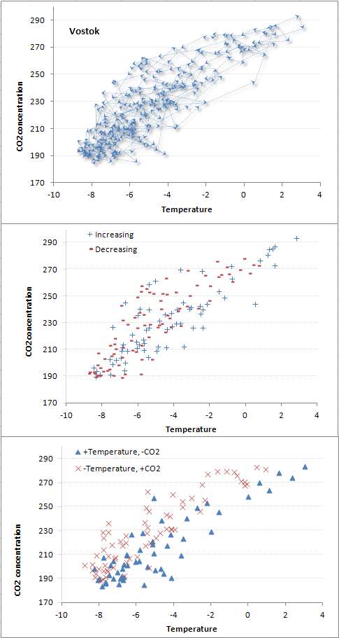
Application. We can use the Vostok ice core data to evaluate the model. My previous posts on Vostok introduced the CO2 outgassing concept and evaluated a few random walk simulations. The following figure gives an idea of the raw data we are dealing with and the kind of random walk simulation one can generate.

To run a simulation,we need to establish a working temperature range, as the absolute temperature is required for the αβ model. Realizing that the actual Vostok temperature range was not known but the relative temperatures were available, I took an arbitrary starting point of 288 K (corresponding to a temperate or warm region). Some value is needed since a T^2 factor plays into the model. Placing the value 50K less will not change the interpretation.
Further, it is clear that a lag between Temperature changes and CO2 changes exists. Historically, there is little evidence that large scale CO2 changes have been the forcing function and something else (i.e. Milankovitch cycles) were assumed to kick off the climate variation. The lag is likely most noticeable on temperature decreases, as it is understood that the long adjustment time of atmospheric CO2 to sequestration is a critical and significant aspect to transient climate sensitivity.
The following figure illustrates both the steady-state αβ model and a lagged CO2 Monte Carlo simulation. The Monte Carlo random walk simulation simply integrates the d[CO2] and dΔT expressions described above, but on temperature decreases I introduce a lag by using the value of temperature from a previous step. This generates a clear lag on the trajectory through the phase space as shown in the following figure.


The simulations are very easy to do in a spreadsheet. I will try to create a Google Docs variation that one can interact with in this space. [I will also configure a scripted standalone simulator so that I can generate thousands of runs and accurately represent a 2D density plot -- this will more clearly show the ΔT versus [CO2] uncertainty. see below]
I am more and more convinced that paleoclimate data is the best way to demonstrate a signature of CO2 on climate change, given the paucity of long time series data from the real-time telemetry and instrumentation era (view the CO2 control knob video by Richard Alley to gain an appreciation of this). I still won't go close to applying current data for making any predictions, except to improve my understanding. Less than one hundred years of data is tough to demonstrate anything conclusively. The paleoclimate data is more fuzzy but makes up for it with the long time series.
Added 2D contour plots:


The background contour densities correspond to more probable state space occupation, assuming a start from the highest density point. Each was generated from a set of random walk simulations averaged over 1000 runs assuming an α value of 5 and a β value of 3500 Kelvins (i.e. Takahashi pCO2 doubling). The lower plot has a slightly lower β value of 3300 Kelvins and has a lag 2/3 smaller than the upper plot.
This is the simple random walk simulation source code that gets fed into gnuplot (corresponding to the lower figure).
srand()
RC = 0.5 ## Scale of hop
a = 5.1 ## Alpha
b = 3300.1 ## Beta
f = 0.3 ## fraction of lag
T0 = 290.9 ## start Temperature
C0 = 226.1 ## start CO2
loops = 1000
while(loops--) { ## Number of runs
T = T0
lastT = 0.00001
C = C0
dT = (1.0+rand())*RC ## Start Noise term
dC = 0.00001
i = 2000
while(i--) { ## Length of random walk sim
dT0 = lastT
dT1 = dT
dC1 = dC
dT = a*b*dT/T/T + (0.5-rand())*RC ## Feedback+Noise
if(dT1>0)
dC = b*C*(f*dT+(1.0-f)*dT1)/T/T ## Lead response
else
dC = b*C*(f*dT0+(1.0-f)*dT1)/T/T ## Lag response
T += dT1
C += dC1
lastT = dT1
## Store random walk location
Histogram[int(T),int(C)]++
}
}
## Collect statistics
for(T=284;T<=298;T++)
for(C=170;C<=300;C++) {
if(Histogram[T,C]>0)
print T ", " C ", " Histogram[T,C]
else
print T ", " C ", " 0
}
References Takahashi, T; Sutherland, SC; Sweeney, C; Poisson, A; Metzl, N; Tilbrook, B; Bates, N; Wanninkhof, R; Feely, RA; Sabine, C; Olafsson, J; Nojiri, Y "Global sea-air CO2 flux based on climatological surface ocean pCO2 and seasonal biological and temperature effects" Deep-Sea Research (Part II, Topical Studies in Oceanography) [Deep-Sea Research (II Top. Stud. Oceanogr.)] 49, 9-10, pp. 1601-1622, 2002
Added per comment:
The following figure shows that Argon levels (the temperature proxy) lagging the CO2 levels .

from Caillon, et al, "Timing of Atmospheric CO2 and Antarctic Temperature Changes Across Termination III"
http://www.sciencemag.org/content/299/5613/1728.abstract
Seasonal Outgassing Model
What we also need is current data from both CO2 and sea surface temperatures (SST) to determine whether we can better calibrate the CO2 outgassing.
- The SST data was taken from a NOMADS server (NOAA Operational Model Archive and Distribution System)
http://nomad3.ncep.noaa.gov/cgi-bin/pdisp_sst.sh?ctlfile=monoiv2.ctl&varlist=on&psfile=on&new_window=on&ptype=ts&dir=
- The CO2 data was taken from the Mauna Loa records, going back to 1981 to match the archival extent of the SST records
http://www.woodfortrees.org/data/esrl-co2/from:1981
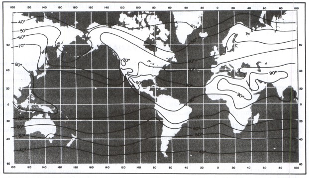
Since the Mauna Loa CO2 shows extreme sensitivity to seasonal fluctuations, I culled the SST data to give the most regional sensitivity to the maximum excursion of CO2 levels. This likely corresponds to the latitudes of maximum temperature, which should give the maximum CO2 outgassing. From the data, the maximally warm average SST exists at around -6 degrees latitude.
 |
| January Temperatures |
 |
| July Temperatures |
The next step was to take a spread of latitude readings +/- 15 degrees from the maximally warm latitude. That spread is somewhat arbitrary but it captures the width of the warmest ocean regions, just south of Hawaii. See the Pacific Warm Pool.


Both the CO2 and SST curves show a sinusoidal variation with a harmonic that generates a side hump in the up-slope, as shown below.

This time, instead of doing a Fourier analysis, I used the Eureqa curve fitting tool to extract the phase information from the SST and CO2 measurements. This is very straightforward to do as one only needs to copy and paste the raw time-series data into the tool's spreadsheet entry form.
Letting the CO2 fit run in Eureqa results in this:

Letting the SST fit run in Eureqa results in this:

I chose the maximal complexity and lowest error result in both cases. Subtracting the trend and offsets from the fit, I was left with the yearly period plus one harmonic to reproduce the seasonal variations. Two periods of CO2 and SST variations are shown below:

Note how well aligned the waveforms are over the yearly cycle. The Mauna Loa measurements have a 0.04 period shift which is a mid-month reading, and I assumed the SST readings were from the beginning of each month. In any case, the lag from temperature variations to CO2 response has an uncertainty of around one month.
In the plot above, the SST readings were scaled by 3.2 to demonstrate the alignment. If we plot the phase relationship between SST and atmospheric concentrations, the transient scaling shows a slope of 3 PPM per degree C change. This is the transient outgassing relationship.

The transient outgassing is much less than the equilibrium number since the seasonal temperature variations prevent the partial CO2 concentration from reaching an equilibrium. So the [CO2] always reflects but slightly lags the current regional temperature as it tries to catch up to the continuously changing seasonal variations. This is the actual spread in the data, removing the lag:

The cross-correlation function shows alignment with 12 month cycles, which is not surprising.

So this phase plot can be compared to the phase plots for the Vostok data, which show a much larger outgassing sensitivity exaggerated by the GHG positive feedback warming mechanisms. The Vostok plot gives a 10 PPM per degree change over the interglacial temperature range.
Added:
The following figure shows two theoretical phase plots for other common soluble gases, Argon and Nitrogen. This is taken from "Continuous Measurements of Atmospheric Ar/N2 as a Tracer of Air-Sea Heat Flux: Models, Methods, and Data" by T. W. Blaine. Note the similarity to that for CO2. The thesis is highly recommended reading as it applies many of the same math analysis, such as the two harmonic fit.

A couple of Wolfram Alpha models for the phased response of [CO2] from a forcing temperature with gain of 3, and an anthropogenic [CO2] ramp included:
First-order response: x + (1/30) dx/dt = 3*cos(2*pi*t) + 2*t

Phase relation from the solution: plot cos(2 pi t) and (675 pi sin(2 pi t)+10125 cos(2 pi t))/(15 (225+pi^2))

The value of the normalized time constant (in this case 1/30) sets the width of the slanted ellipse. The smaller that value is, the narrower the ellipse becomes.
ADDED 2013
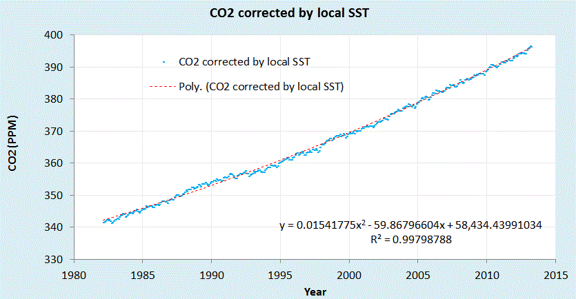 |
| Corrected Mauna Loa CO2 data |
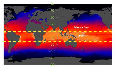 |
| The Indo-Pacific Warm Pool (IPWP) lies within the +9N to -21S SST average |
We can do the same for another CO2 reporting station in American Samoa.
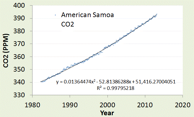 | |
| American Samoa is located in the middle of IPWP (near the label in the map). Very little fluctuation in CO2 is observed since the temperature is seasonally stable on that latitude. |
 |
| This is the carbon emission data convolved with the CO2 sequestering Green's function, sandwiched between the Mauna Loa and Samoa data. The carbon emission data is very smoothly varying after the convolution is applied so a very slight additional temperature-dependent CO2 outgassing based on filtered global SST is added. This is slight as shown in the next graph. |
 |
| If we take the residuals from the polynomial fitted curves (including one for the carbon residuals from the CDIAC, see chart above) we see how well the curves agree on a year-by-year basis. All this really shows is that the residual is at best +/- 1 PPM which may be due to additional global SST variations (the yellow circles) but could also be any disturbances (such as volcanic, biotic, wildfires, etc) as well as possible systemic (measurement) errors. |
The entrapment of Ar in the ice is a much better proxy of ocean temperature than CO2. So far there are only a few ice core measurements, but these do show Ar outgassing (via the Ar/N2 ratio), with no chnage in CO2.
ReplyDeleteAr, unlike CO2, is non-biotic and one can see that CO2 levels do not track temperature.
The Argon 40 level is used as the proxy for the Vostok temperature. That much is of course assumed, and I included the reference which estimated the 800 year lag.
ReplyDeleteDocMartyn has a theory that all changes are due to some biotic process drawing from iron dust being deposited from outer space. So I am not at all sure what he is getting at, other than to provide some FUD, and perhaps imply that CO2 changes are due to some biological origin as iron is an important nutrient for plant growth.
I hope you don't mind a general question: how might an engineer like me with a strong technical but poor statistical background pick up the basics of the sort of analysis you do? Specifically I'm interested in learning the basics of applying the maximum entropy principle and chaos theory (if the latter is relevant) to my own work.
ReplyDeleteYour posts are fascinating but largely over my head. Are there books that you'd recommend to pick things up? (I assume it'll take three or four books of progressive difficulty at least before I can understand your posts.)
Read up on books by E.T. Jaynes, Murray Gell-Mann, David Mumford, (and also Didier Sornette if you want to get completely over your head) and N.N.Taleb (if you want to get more opinionating).
ReplyDeleteIt looks to me like the δ40Ar peak occurs before the peaks in CO2 and CH4. The x axis is years BP, i.e. going to the right is going back in time. CO2 and CH4, as expected lag temperature, not the other way around. I can't imagine a physical model that would cause CO2 and especially CH4 to increase before temperature increases.
ReplyDeleteDeWitt,
ReplyDeleteYou are right. Except for the initial stimulus, perhaps a volcanic burst or vegetative belch of CO2, it should lag T.
Recent papers are tightening the lag:
[1]J. B. Pedro, S. O. Rasmussen, and T. D. van Ommen, “Tightened constraints on the time-lag between Antarctic temperature and CO2 during the last deglaciation,” Climate of the Past, vol. 8, no. 4, pp. 1213–1221, Jul. 2012.
hoop jumping test
ReplyDeletethis CO2(T) question has been bugging me for a while and I wanted to take an ODE approach. I think this sort of engineering approach is long over due.
ReplyDeleteSeems like you have already done a lot of it.
However, I see in your Monte Carlo plots that model curves the wrong way. The data clearly rises early and flattens out, so I don't think this is a question of return to mean adjustments. It's not bad but there's a basic flaw in the model. A too strong temp dependence.
I looked over this initial equations and I think I see an error.
d[CO2]∼dp=β/T^2.pdT∼β/T^2 . [CO2]dΔT
here you substitute dT with dΔT but not in T^2 term.
this should be (ΔT)^2 , if you work that though as difference of two squares, you get 2T.ΔT in place of T^2
I suggest you modify you ODE accordingly and see if the model matches any better.
regards, Greg.
I'm also a little uneasy about the liberal swapping between dΔT and dT and dΔ[CO2] terms.
ReplyDeletearen't these double diff terms?
Maybe I''m just missing a substitution that you have not laid out explicitly but it seems that there is some inconsistency there too.
d2(T) = d2(C) . [ α - 2βT.dT ] ??
ReplyDeleteOK, I've seen what you've done the T^2 etc, look correct to within usual approximations.
ReplyDelete" liberal swapping" seems to be lack of care and consistency in notation but maths looks correct w.r.t various substitutions.
Perhaps you could explain why second difference terms get muted to single differences in the 'casting' set.
We next cast this in terms of a differential equation where dc=d[CO2] and dT = dΔT.
ReplyDeleteSo the solution you have derived is that between d[CO2] and dΔT.
As I showed in recent data this is in phase and close to linear in agreement with your model.
http://climategrog.wordpress.com/?attachment_id=233
Yet you are comparing to CO2 and T from Vostok. which as we see has a large time lag seen in the Lissajous figures.
Apples and oranges?
Slight correction, what you have solved is for [CO2] and ΔT
ReplyDeletehttp://climategrog.wordpress.com/?attachment_id=223
So, I wonder if the buffering in oceans as carbonic acid, and its being pH dependent throws any kind of a wrench into this thinking. I remember a problem in a problem set (possibly from Ray Pierrehumbert's PRINCIPLES OF PLANETARY CLIMATE, although I cannot find it) which asked the student to calculate rate of CO2 outgassing from oceans as a function of temperature. The time for significant outgassing at present temperatures was large, and the rate only increased slowly with temperature.
ReplyDelete